There always seems to be a steady stream of proposals for changes to TCP congestion control. Here are some issues that are known (sometimes after painful experience) to be be problematic:
1. Making the rate of cwnd increase depend on cwnd (or average cwnd)
To get better scaling across a range of path bandwidth-delay products (BDP), it is often appealing to make the rate at which cwnd increases/probes for bandwidth change with the path BDP. The problem is that of course a flow doesn’t know the true path BDP and so has to estimate it somehow. Its tempting to use the flow cwnd for this – after all a large cwnd certainly means the path BDP is large. The problem is that a small cwnd does not mean that the path BDP is small, it might just mean that the flow has recently started or that bandwidth is being seized unfairly by a competing, more aggressive flow.
As a result, making the cwnd increase rate depend on cwnd (or on average cwnd) is very likely to make network convergence slow or maybe even non-existent. Why do we care about convergence ? Lots of reasons, for example slow convergence can heavily penalise shorter flows and create “race” conditions where the first flow to start can gain a prolonged advantage over other flows.
Examples (taken from this 2007 paper)
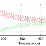 High-speed TCP (slow convergence) |
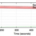 Scalable TCP (unstable) |
2. Throughput and cwnd are not the same
In other words, don’t ignore network buffers. Both large buffers (e.g. DSL and wireless links very often have several seconds worth of buffering) and small buffers (a few dozen packets) are common in modern networks, so don’t design a TCP algorithm that only works with one or the other. Examples: much of the discussion on concave/convex cwnd increase shape is fundamentally flawed since its equates the area under the cwnd time history with flow throughput. To see that this is plain wrong, take the simplest example of a link with a single flow. If the link is backlogged (which TCP’s congestion control generally aims to achieve) then the flow throughput is equal to link rate regardless of how the flow cwnd evolves.
Example (taken from this discussion paper at PFLDnet 2008):
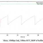
Illustrating that cwnd and throughput are not the same
In general, by adjusting the flow AIMD backoff factor it looks like we can always decouple throughput from cwnd shape. There’s an extended discussion of this point in this paper.
3. Decreasing the cwnd backoff in AIMD can slow convergence dramatically
It is very common to propose changes to the backoff factor used in AIMD – typically to reduce the amount that cwnd backs off and make flows more aggressive. Be aware that the choice of backoff factor can dramatically affect the convergence rate of TCP.
It easy enough to see this by a thought experiment. Suppose one TCP flow is running and a second starts up. What is the mechanism that allows the new flow to grab bandwidth from the old flow ? Well, on loss the flows backoff their cwnds in proportion to their cwnd sizes, so that flows with larger cwnds (the first flow) back off by more than flows with smaller cwnds (the newly started flow). Since both flows subsequently increase cwnd at the same rate (at least if they have the same RTT, but that’s another days work), at the next loss event the first flow will have a lower cwnd than before and the second flow a higher one until eventually the flows have the same cwnd. If we decrease the amount that flows reduce their cwnds, then its no surprise that it will take longer (maybe a lot longer) for new flows to gain bandwidth. For more details/analysis, have a look at the papers here and here.
Examples
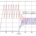 0.5 backoff |
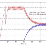 0.9 backoff |
4. Be wary of using fluid models in drop-tail networks
Fluid models are appealing and powerful. However, they often make the basic assumption that flows sharing a link see the same “price” or loss probability. Since the loss probability is per packet, this means that there is an assumption built in that flows with higher rate see a greater number of losses than flows with lower rate. This seems natural to postulate, and is the usual source of stability in fluid models (differential numbers of packet losses penalise flows with higher throughput and creates pressure for the network to converge to fairness).
Unfortunately, when drop-tail queueing is used (and it seems to be ubiquitous in real networks) then more often than not this is simply not true. That is, the number of packet losses seen by a flow is generally not proportional to the flow rate. I’ll post measurement data I have on loss rates some time, but there’s actually a more dramatic demonstration. Early analysis using fluid models suggested that Scalable TCP (which increases cwnd exponentially rather than linearly) is stable. However it is now known (e.g. see Ethan ltman’s MIMD paper) that in drop-tail networks Scalable TCP is in fact unstable, and in what seems like the worst possible way e.g. in a network with flows having different round-trip times (RTT), the flow with the smallest RTT seizes all of the bandwidth, leaving all the other flows starved. This happens even for very small differences in RTT. When flows all have the same RTT, there exists an infinite number of equilibria and the allocation of bandwidth between flows is basically a random function of flow start times.
A second warning example is that of RTT unfairness predictions. Fluid models, including Padhye “bath of noise” type models, predict that throughput unfairness is proportional to 1/RTT. However, in drop-tail networks many measurements exist (plus analytic models targeted at drop-tail links such as the one here) tell us that throughput unfairness seems in fact more like it is proportional to 1/RTT^2. Again, the source of the discrepancy is the assumption that flows sharing a link experience the same loss probability.